Introduction
The possibility of world-wide F-layer propagation is a particularly intriguing
part of the challenge of six-metre operation. Even the casual six-metre operator
will soon notice that there are some fairly mysterious things going on when
it comes to ionospheric propagation. The more seasoned operator will notice
that there are a number of patterns that are prevalent, but it is still very
difficult to predict when the band will open, especially on a day-to-day
basis. Unfortunately, there are no simple answers to this dilemma. Nevertheless,
there are some pieces to the F2 puzzle that are known and understood, and some
clues to those that remain mysterious. In order to understand (however imperfectly)
when the band will open, it is essential to have some understanding of why the
band will open.
A discussion of why signals propagate has to begin with some basic facts about how radio waves behave in the ionosphere. There are three basic elements that critically effect this propagation:
1. The amount of ionisation present,
2. The angle of attack of the incoming signal to the ionosphere, and
3. The presence of large or small irregularities in the ionisation.
These factors play key roles in the success or failure of a communications path via either E or F layers. Although there are many external things that influence the status of the three conditions, in the end, it is the combination of these three that make or break any path. The way in which external events effect these three parameters determines what kind of propagation will occur.
Six-metre F2 propagation is a very improbable event, from a statistical point of view. While this may seem obvious, it has a very important consequence. `Unlikely' events in complex physical systems are often the result of a combination of factors, some of which also may be fairly unlikely. This is certainly the case with most six-metre F2 activity, where propagation is almost always at or very near the ultimate edge of what is possible.
The task of predicting band openings generally involves predicting not just
one event, but the coincidence of several events, and not always the same ones
or in the same combinations. In truth we do not yet know what all of the factors
are, much less how they interact. On the other hand, there are a number of things
that are known to be significant and most of them involve the Sun in one way
or another.
The Ionosphere and the Sun
The Earth's atmosphere extends from the surface to heights well in excess of
1,000 km. The density of the static atmosphere is highest near the surface and
decreases progressively as one goes upwards. Most of the atmospheric mass is
located very near the Earth's surface, with more than half of the mass contained
within just the first 6 km.
The Sun, on the other hand, pours its radiation down on the atmosphere from the topside. Thus, the upper regions of the atmosphere receive the full brunt of the Sun's ultraviolet, X-rays, cosmic rays, and so forth. This radiation interacts with the atmosphere on its way down, and as it does, portions of the radiation are absorbed at different levels, producing ionisation in the process.
The interactions between solar rays and the air molecules and atoms are
very complicated. There is a whole complex
of chemistry that can take place at these rarefied heights that normally has
no importance at lower levels. What wavelengths are absorbed at what levels
is determined in part by the chemical components and particle densities found
at each level. For example, generally ultraviolet radiation is absorbed
fairly high in the atmosphere, while X-rays penetrate somewhat lower, and
cosmic rays go still lower.
When solar photons get absorbed it is a result of a collision with an atom or molecule. Often such collisions occur with sufficient force to knock off one or more electrons from the atom or molecule struck. This leaves behind a missing (absorbed) photon and positively and negatively charged ions. Usually the positive ions are the comparatively heavy cores of the atoms or molecules and the negative ions are the relatively light electrons. It is the electrons that play the dominant role in radio propagation.
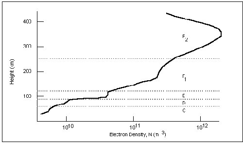
Figure
1. A typical plot of the daytime electron density as a function of height above
the ground, showing the C, D, E, F1, and F2 layers.
Since different wavelengths are absorbed at different heights, the
solar radiation leaves behind several distinct layers that are
characterised by enhanced levels on ionisation.
The F2 layer is the highest of these, both in terms of distance above ground and
in terms of electron density. This layer extends from roughly 250 km above
the Earth to well over 500 km on occasion, with a peak daytime electron density
in excess of 1012 e/m3 around 350 km.
Extreme-ultraviolet radiation (EUV) from the Sun
is the main source of ionisation in the F region. Table 1 below shows
typical characteristics of the various layers. It should be noted that the
`boundaries' between the layers are ill defined
and for sake of brevity the list of ionising radiation is not entirely complete.
| Layer (km) |
Height (e/m3) |
Density Radiation |
Ionising |
| C | 30 - 60 | 5x10¹⁰ | Cosmic Rays |
| D | 60 - 90 | 1x10¹⁰ | Hard X-rays |
| E | 90 - 120 | 8x10¹⁰ | Soft X-rays |
| F1 | 120 - 250 | 5x10¹¹ | Extreme Ultraviolet |
| F2 | 250 - 500 | 3x10¹² | Extreme Ultraviolet |
Ionospheric Radio-Wave Propagation
The Amount of Ionisation - When an upward moving radio wave reaches the
ionosphere, the electric field in the wave forces the electrons in that layer
into a sympathetic oscillation at the same frequency as the passing wave.
A certain amount of the wave energy is given up to this mechanical vibration of the electron cloud. As a result, the passing wave gets weaker. At this point there are two sorts of things that can happen. In the lower atmosphere, the total number of particles may be high enough that the oscillating electrons collide with other particles almost immediately (say, in less than one RF cycle). When that happens, the wave energy that was converted to the mechanical electron oscillation is now converted as heat to the atmosphere before anything else can happen. This energy is lost forever as far as the wave is concerned. This is another way of saying that the radio wave energy is absorbed.
This is precisely what happens to signals below about 10 MHz when they encounter the daytime D layer. The average daytime frequency of collisions between particles in this region during the day is about 10 million collisions per second. So, it strongly absorbs radio frequencies below 10 MHz, but has a progressively smaller effect as the frequency gets higher.
At the other extreme, if the collision frequency within the layer is significantly less than the wave frequency, and if the electron density in the vibrating cloud is greater than a certain critical value, then the whole cloud can act more like a static reflector. Almost all of the wave energy is given up to the vibration in a very short distance, all the electrons vibrate in phase, and together they reradiate the original wave energy back downward again. Thus, the wave skips off the ionospheric layer, hopefully to be received at some distant point.
It should be noted that in most cases what actually occurs is something intermediate
to these two extremes. Some amount of absorption always occurs. Moreover, as
Figure 1 shows, when the electron density does exceed the critical skip value,
it does so gradually. Rather than a discontinuous reflection, there is a refraction
of the wave, a more gradual bending back around toward the ground (sporadic
E is an exception, it is usually very close to a true reflection).
Even when the critical density is not reached (and the wave passes through
the ionosphere and escapes into space), a certain small fraction of the wave
is re-radiated by the vibrating cloud and some of this new signal goes downward
as a form of ionospheric scattering.
Let us consider the electron density, and ignore other effects for the moment. If a radio signal is sent straight up, one can calculate the critical frequency, fc, the highest frequency that the ionosphere can reflect that signal straight back down as
Here, N is the number density of electrons, e is the electron charge, e0 is a number called the permitivity of free space, and m is the mass of the electron. Everything except N is a known constant value. The real point here is not the mathematics, but the basic fact that the highest frequency that will skip straight back down vertically is the square root of the electron density times a fixed number. So, for example, in order for a signal to skip at twice the current maximum frequency, something must increase the number of electrons by a factor of four.
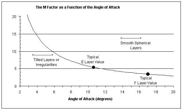
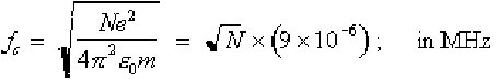
Figure 2.
M varies with angle of attack. A smooth spherical ionosphere gives angles between
10 and 20 degrees. Lower layers lead to smaller angles, larger Ms, and higher
MUFs, for same ionisation. For VHF, tilted layers or other irregularities can
produce angles below 10 degrees and provide very exciting results. In the extreme,
TEP on 222 MHz and higher can result.
Notwithstanding the fact that the F2 layer retains some of its ionisation even at night, all of the foregoing should make it clear that six-metre F2 propagation is normally a daytime affair, unless one lives in the tropics (but more on that later).
The Angle of Attack - The above example only tells us what happens if the path of the wave strikes the ionosphere with an angle of attack** of 90° (i.e. going straight up). In the more general case, if skip is to occur, the Maximum Usable Frequency (MUF) that will bounce is determined by both the maximum electron density that the wave encounters in the ionosphere and the angle at which the wave hits the reflecting/refracting layer.
If a signal that is sent off very near the horizon (that is, with a zero angle of radiation), due to the curvature of the ionosphere around the Earth, the signal will normally hit the ionosphere at an angle of attack between 10° to 20°. The exact value depends on the height of the ionospheric layer and exact angle of radiation. The MUF (represented by fmax) can be calculated from:
where a is the angle of attack. Here one sees the dependence on both the electron density and the angle a. The cosecant term is often referred to as the "M factor".
Radio propagation is not the only place one sees grazing-incidence reflection effects. For example, everyone knows that if you toss a rock in a lake it will break through the surface of the water and sink, never to be seen again. The same thing happens to a radio wave when it collides with the ionosphere and its frequency is above the MUF - it breaks through and disappears.
However, even a rock can be made to bounce off the surface of the lake - any child can do it. The secret, of course, is that it must hit the surface at a very shallow angle, that is to say, at grazing incidence. Skipping radio waves is essentially the same as skipping stones.
If the ionosphere were a smooth sphere, simple geometry would show that M ~ 3.4 at the F2 layer. Since Table 1 shows that the average E-layer ionisation is 40 times less than the F2 layer, one might rightly wonder why sporadic E propagation is so much more common and frequently produces much higher MUFs than the F-layer.
Half of the answer is that the E layer is closer to the Earth making the angle of attack much smaller than for the F layer. At E-layer heights, Figure 2 shows that M ~ 5.4. Thus, the E-layer MUF will be nearly 60% higher than the F layer for the same number of electrons. (The other half of the ES story is that the `sporadic' process also increases the amount of ionisation in thin localised regions to levels considerably higher than the average in the E layer as a whole. These two effects can produce very high E-layer MUFs.)
It is important to note that the angle of attack is also effected by
the radiation angle of the antenna. Especially at six meters where one is struggling
to get the MUF up high enough, a low angle of radiation from the antenna can
be very important. Here, it is not just a matter of getting the longest skip
distance, but one of getting any skip at all.
F-Layer Propagation for All Seasons (Except Summer)
The amount of ionisation in a given layer at a given time depends on the dynamic
balance between those processes causing ions to be produced and those causing
ions to be lost (e.g. by returning to their original neutral state). Put another
way, the ion density depends on the amount of radiation arriving from the Sun
causing the production of ions, minus the loss of ions due to electrons
being recaptured by positive ions. The rates and mechanisms of these processes
vary widely from layer to layer.
For example, the underlying (neutral) density of the D layer is much higher than that of the F layer. Consequently, in a given length of time, electrons and positive ions there are much more likely to collide and recombine. As a result, by comparison to the F layer, the maximum D-layer ionisation is held down during the day by collisional losses, and the D layer disappears in minutes when the Sun goes down. By contrast, the underlying particle density in the F layer is much less than the D layer and ions last a lot longer in the F layer. Even late at night, often there are enough ions left to support HF communications.
Another important effect in ion production is the angle with which
the sunlight strikes on the top of the Earth's atmosphere. When the rays
arrive at a large angle to the vertical the energy is spread out over a larger
area, and thus the energy density at any one
spot is reduced. So, fewer electrons are produced at sunset and sunrise than
at high noon. In addition to this diurnal effect, there is a seasonal one as well.
The local winter hemisphere is tipped partly away from the Sun and its
various layers receive proportionately less radiation. Consequently, in the
Northern Hemisphere fewer daytime F-layer electrons are produced at a given
time of day in January than are produced in July.
However, remember that production is only half the equation. There is a peculiarity in the F2 layer, not found in the other layers, called the winter anomaly. Although daytime ion production is higher in the summer, there are seasonal changes in the molecular-to-atomic ratio of the underlying (neutral) atmosphere that cause the summer ion loss rate to be even higher. The result is that the increase in the summertime loss overwhelms the increase in summertime production, and total F2 ionisation is actually lower, not higher, in the local summer months. Put the other way around, daytime F2 electron densities, and thus MUFs, are higher in the local winter.
Measured at the `half-width', the winter peak starts in October and lasts until
May or June. Most years there is a fairly flat peak between December and April.
It is interesting to note that during the peak years of solar cycles 18 through
21, October was almost always the beginning half-maximum, whereas the ending
half-maximum varied from April to July. The ending months were pretty consistent
within a given cycle, but cycles with higher maxima favoured May with an occasional
April, while those with lower maxima favoured June with an occasional July.
Figure 3. A schematic plot of the Northern Hemisphere variations of MUF due
to the winter anomaly. The values of MUF shown are typical mid day figures for
mid latitudes near solar maximum.
Interestingly, the winter anomaly shows the most seasonal fluctuation
near solar maximum. Here the local winter daytime MUFs are twice as high as
the daytime summer values, while they are only about 20% higher during solar
minimum. The central message in all of this is that, on average, F2 propagation
between points on the same side of the
equator will be much better in the local winter and near solar maximum.
If one is interested in multihop along generally north-south paths, then the winter anomaly comes into play in another way. If it is wintertime in one hemisphere, it will be summertime in the other. So, for example, in January the first hop of a two-hop path from North to South America might make it, only to have the second hop fail due to the absence of the winter effect at the second skip point. Obviously, the best times of year for such a path would seem to be in the Fall and Spring when the winter anomaly effects overlap a bit in both hemispheres.
The winter anomaly is not the only seasonal effect. Many two-hop (or more)
north-south openings on six metres seem to have no evidence of stations at the
end of the first hop. This is often due to the ionospheric equatorial
bulge known as the equatorial anomaly. Within ±20° of the Earth's
magnetic equator there is a pronounced outward bulge in the ionosphere.
Though generally regarded as an afternoon or early evening phenomenon, it occurs
at other times as well. It is thought to be produced by a combination of a persistent
thickening of the F layer near the equator and a daily fountain effect.
This afternoon fountain apparently is the result of a build up of west-to-east
electric fields in the equatorial E layer. In combination with the Earth's magnetic
field and ionospheric winds, these fields pump electrons upward from the E and
lower F layer into the upper F2 layer. Thus, significantly enhancing F2 layer
electrons.
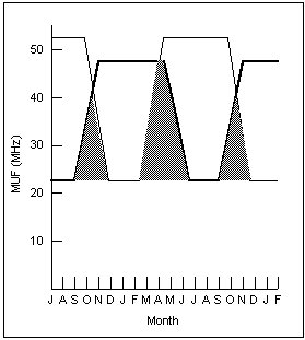
Figure 4. A schematic of the overlap of the northern and southern winter
anomalies in the western hemisphere, as modified by the effect of the (magnetic)
equatorial anomaly. The shaded areas show the most likely times for mid latitude
north-south transequatorial multihop.
It was pointed out earlier that the angle with which the radio wave encounters the layer is also a factor in determining the MUF. The equatorial bulge produces two regions, one north of the equator and the other south, where the ionosphere is systematically tilted. Of particular interest are the points at the corners where the generally spherical ionosphere is bent upwards to form the bulge.
This upward tilt is such that an upcoming wave hits the near corner at a
shallower angle of attack to the tilted layer than it would to the usual spherical
layer. This means that it will have a higher MUF for the same value of electron
density. That is, the M factor is larger than 3.4, perhaps by quite a bit. The
wave is not bent all the way back toward the ground. However, it is bent enough
to cross the equator and hit the tilted layer on the far side, without ever
coming back to Earth.
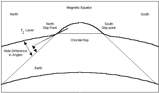
Figure 5. A diagram of a transequatorial chordal hop off the tilted north
and south skip points. These points lie about 20° north and south of the
Earth's magnetic equator and can be major contributors to daytime transequatorial
six-metre propagation from mid latitudes and clearly cause night-time TEP in
the tropics.
This so-called `chordal hop' to the second tilted region produces another small-angle reflection that can be just enough to return the signal to the Earth on the far side of the equator. The effect is a kind of double hop with nothing in between, and at a higher MUF than could otherwise be supported. Since the `bulge' effect does produce higher MUFs, this is often the cause of multi-hop north-south propagation of six metres. Moreover, it is a fairly low loss path. The wave never comes down at the path midpoint, so it avoids two passes of D-layer absorption that normal double hop would have encountered.
In order for this form of propagation to function, both the north-side and south-side tilted regions need to be ionised enough to make the path work. Again, if either one is insufficient to skip then the whole path fails. At HF there is often a fair amount of margin, but not at six metres. Here usually the best chance occurs when both sides of the equatorial bulge are equally illuminated by solar radiation, and this situation only occurs around the autumn and spring equinoxes when the Sun is most nearly over the equator.
Normally one would think that this would occur in late September and late March. However, the Earth's magnetic field is tilted with respect to the geographical co-ordinates. In the Western Hemisphere the magnetic equator is as much as nearly 11° south of the geographic equator. This means that the `magnetic equinoxes' occur about a month or more earlier (August and February) for paths between North and South America. From the point of view of a station in North America, as the path of interest swings around further east or west, the magnetic equinoxes are more nearly the same as the geographical ones. Consequently, the date of the magnetic equinox is dependent on the amount of east or west component included in the north-south path, and where you happen to be on the Earth.
There is also an interaction between the balanced illumination at the magnetic equinoxes and the double-hop winter anomaly effect (which is geographical, not magnetic). For example, consider a path between North and South America. Here it should be noted that, in part as a consequence of the location of the magnetic equator, MUFs are frequently higher over South America than North America. During the Fall equinox period, on the northern side of a path, August is too early for much help from the (northern) winter anomaly. By contrast, the southern skip point is bolstered by both the winter and equinox effects and has a substantially higher MUF than the northern point. If this path is going to succeed it will likely have to wait until October when the northern skip point is in better shape. Put another way, by October the northern and southern skip point MUFs will be about the same, as they pass each other going in opposite directions.
During the Spring period, February, as well as March and April, are all still in the peak for the north end. Even though the southern point is in the summertime, it has a higher MUF to begin with, and the equinox effect adds even more. The result is that the southern point MUF may well be higher than the northern point MUF, despite the absence of help from of the winter anomaly. In the meantime the northern point is as good as it will ever get, because of the winter anomaly. Consequently, for generally north-south paths across the magnetic equator between North and South America, periods more nearly centred on October and March are generally the best, and often the Spring gives more consistent daytime transe-quatorial performance.
Of course, unless one has an E-layer link up, or some other funny business, another requirement is that the stations each be close enough to the nearest ±20° tilted skip point to illuminate that point by radio line of sight. Based purely on geometry, the southern half of the U.S. has an advantage for South American paths and the south-western states for the South Pacific. (Early spring sporadic-E can make a big difference on the mainland US.)
The Solar Cycles
For reasons that are still unknown, the general background magnetic field of
the Sun reverses polarity every 11 years or so. Thus, the Sun experiences a
22-year magnetic polarity cycle of north to south to north again. This effect
is accompanied by a cycle of solar activity that reaches a peak approximately
every eleven years. The peak itself can be fairly broad, having significant
effects for three or four years.
The solar activity cycle is seen in virtually every kind of signal we can receive from the Sun, from radio waves to X-rays. Not surprisingly then, the amount of ionising radiation impinging on the atmosphere varies with this same pattern, including the EUV that is the principal source of the F2 layer. Consequently, propagation is decidedly better near solar maximum, but the seasonal effects are still superposed on the general enhancement seen during the solar maximum.
There is a second kind of variation due to the fact that the Sun rotates on its axis every 27 days or so, coupled with the fact that `activity' on the solar surface is generally confined to a few specific regions at any one given time. As a result, if the Sun is active at all, it is quite common for one side to be active and the other side relatively quiet. As the Sun rotates there is often a very pronounced 27-day cycle in the radiation reaching the Earth.
It should be noted that the active solar longitudes change over time. The 27-day cycle of activity commonly repeats for several cycles and then briefly is interrupted as old solar active regions fade and others emerge. When new active regions do develop, typically at some other longitude, the cycle will be re-established, but with a different phase. In other words, knowing that a particular two-week period was active last month is a pretty good predictor that the same two-week period this month also will be active. However, it is a very poor predictor of activity during the corresponding period six months from now.
There is no doubt that during solar maximum, and especially during periods of high activity, the amount of EUV reaching the ionosphere increases substantially. In principle, this should mean better propagation. People have tried for some time to get direct measurements of the EUV radiation with an eye toward making short-range predictions of propagation conditions, but so far these have not been very successful.
Very little of the F2-producing EUV reaches the Earth's surface, precisely because it is absorbed making ions in the F layer. A number of spacecraft have carried EUV sensing instruments, but generally these detectors are susceptible to damage from the very radiation they wish to measure. As a result, their sensitivity changes in time, making accurate, long-term, absolute measurements very difficult to get.
For many years scientists have been using the 10.7-cm solar radio flux as a proxy for EUV emission. This radiation is formed at about the same level in the Sun as the EUV, and has similar temperature sensitivity. Under relatively quiet solar conditions the 10-cm and EUV fluxes track pretty well.
However, there is a component of the 10-cm emission that is also sensitive to other forms of activity including those that produce X-rays. Consequently, during periods of high activity 10 cm is not a good linear indicator of the strength of the EUV radiation reaching the F layer. In fact, it tends to overestimate the EUV considerably.
It must be said that while the 27-day effect definitely influences propagation through flares and such, many people (including the author) think it is not as profound as is generally thought.
There is a good correlation between the long-term average of the 10-cm flux and F2 propagation (as there is with sunspots, flare counts, and many other activity measures). Thus, if the flux is high on average, month after month, propagation will probably be good. However, vertical incidence ionograms show virtually no day-to-day correlation between 10-cm fluctuations and the measured critical frequencies (fc's) that would signal the expected MUFs.
This is not to discount keeping track of the 10-cm flux; it is a
useful indicator of the general level of solar activity. Unfortunately, during
solar maximum one never knows whether high flux numbers mean high EUV and high
F-layer MUFs, or high X-rays and high D-layer absorption. It is certainly
true that long periods of time with high flux
numbers will contain periods of good propagation, but it is very hard to
say whether the openings will come on individual days when the flux is 300
or on days when it is 150. The individual days with high fluxes are a lot
less important than whether there were some days with high fluxes within the
last 30 to 40 days.
Other Solar Effects
Perhaps the most talked about solar events are flares. These more or less
random high-energy outbursts produce a variety of effects, and no two flares
are ever exactly alike. Flares generally occur in active regions and, if they
are to effect the Earth, the active side of the Sun must face the Earth. To
this extent they are weakly predictable.
There is also a mysterious 157-day period associated with flares, and most other solar activity measures, that so far has been ignored by most propagation prognosticators. Some suspect that this is related to a periodic effect in the emergence of new active regions on the Sun and the resetting of the phase of the 27-day cycle.
The impact of solar flares is very unpredictable. Generally there is a large outburst of X-rays associated with big flares. This usually produces an almost immediate increase in both the amount and maximum frequency of D-layer absorption. This often results in widespread `blackouts' of the HF spectrum on the daylight side of the Earth that may last for many hours.
There may also be outbursts of EUV in some flares that produce a very rapid response in the F layer. However, while the x-ray flux may change by a factor of 100 or even 1,000 in a major flare, the EUV may only go up by a factor of 2 to 5. Sometimes excellent six-metre openings do result from a flare, provided that the D layer does not get in the way (it generally does not). At other times flares seem to hurt rather than help.
Of course, another possible effect of flares is geomagnetic disturbances.
All flares blow some material away from the surface of the Sun. If the trajectory
of this material takes it to the Earth (it often misses), then it will arrive
within a few hours to a couple of days and may produce profound disturbances in
the geomagnetic field. This can be either good or bad for F2 propagation.
Whatever the conditions were before the par
ticles arrived, it often means things will then
change.
Storms effecting the F layer often have a positive and then negative
effect on the electron densities, and hence the MUF, on a time scale of several hours.
At mid latitudes, electron densities can climb as much as 20% above the
ambient and then drop to 30% below the ambient all over a period of 24 hours or less.
On the other hand, in equatorial regions a general enhancement of 5 - 10% is
often seen, with no pronounced negative effect.
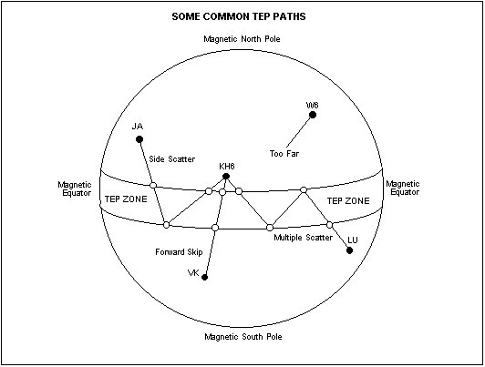
Figure 6. In geomagnetic coordinates, Hawaii is nearly due north of Australia
and these TEP paths transverse north-south paths often behave like conventional
skip. Signals are usually clean and stable. East-west signals from Japan and South
America commonly have heavy scatter modulation, at times resembling aurora, and
display Doppler effects as well.
Transequatorial Propagation (TEP)
Large-Scale Irregularities - One of amateur radio's many propagation
discoveries was that stations located close to the magnetic equator are often
able to communicate at 50 MHz by way of the F layer in the dead of night, over
long paths that cross the magnetic equator. The basic mechanism is the equatorial
anomaly discussed earlier. That is, the afternoon fountain effect causes enhanced
electron densities and tilted layers to form within 20° of the magnetic
equator late in the day or early in the evening. These conditions can persist
long into the night with some contacts taking place long after local midnight.
They readily provide near grazing-incidence chordal hops at six metres.
For operators who have the good fortune to be in the TEP zone, the paths themselves
do not have to be especially north-south. In the simplest case, the two stations
are on opposite sides of the magnetic equator, although they can be at a considerable
angle to the north-south line. All that is necessary is that the two ±20°
corners be at usable chordal skip points.
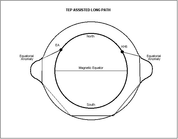
Figure 7.
TEP can provide the launching points for shallow attack angle grazing hops that
cover long distances, with higher than normal MUFs and low absorption. At such
times, long-path can be a superior mode of propagation.
In reality, many contacts are made using TEP, a form of side-scatter mode. If
the two stations are substantially east or west of each other (in geomagnetic
co-ordinates) their signals will enter the region between the two chordal skip
points at a considerable angle to a north-south line. When this happens, the
signals can bounce back and forth within the north and south walls of
the equatorial bulge, using the bulge as a duct.
As depicted in Figure 6, signals can be thought of as zigzagging north and south in the short term, but generally moving along in an east-west direction under the bulge until they find a weak point and break out. From there, they may go either north or south, depending on which side they find the `door' out, irrespective of whether the signal originally entered the duct from the north side or the south side.
Typical examples of across-the-equator TEP include the night-time pipeline that often exists between Hawaii and Australia. Geomagnetically, this is essentially a north-south path. Usually signals are pretty clean, and quite strong.
On the other hand, it is not that uncommon for Hawaiians to hear Japan at the same time - and on the same beam headings as Australia - on what sounds like backscatter. Japan and Hawaii are on the same side of the equator and mostly east-west of one another.
Finally, propagation across the equator, but largely along the TEP zone, can produce very strong signals, such as the link between Hawaii and South America. However, many times these signals are strongly modulated indicating significant scattering within the duct.
Long Path Magic
Nothing illustrates the effect of the angle of attack better than long-path
(wrong-way) propagation. At first glance one might expect that long-path links
would be doing it the hard way. However, this is not always the case. No matter
which direction one points an antenna, if the path goes at least half way around
the world, one is assured of crossing the magnetic equator at least once. Consequently,
there is at least one opportunity for a chordal hop, with its elevated MUF and
absence of D layer absorption.
More importantly, if the chordal hop is at the beginning of the path, then the signal may be injected into the ionosphere at the end of the hop at a very shallow angle. If it is shallow enough, it will continue skipping around the ionosphere in a series of short grazing-incidence hops, as described in Figure 7. Although it can happen at any latitude (especially if aided by, say, a sporadic-E link up to the TEP zone), stations within the TEP zone itself have the most frequent opportunities to experience this kind of propagation.
Consider the case of a path starting in Hawaii and ending in Spain. The long-path link passes south-west from Hawaii, over Australia, Antarctica, Africa, and finally to Spain. The key factor here is that the first and last hops are off the equatorial bulge.
If conditions are right at both ends (and in the middle) the chordal hop might be shallow enough that, when bouncing off the southern edge of the anomaly, it never comes down to Earth. Instead it continues to bounce like a rock skipping across a lake as the curving ionosphere keeps coming back to meet it again.
If the same conditions exist at the magnetic equator over Africa, as those south of Hawaii, the shallow skipping wave will finally be bounced down out of the ionosphere by the northern edge of the bulge, landing in Spain. Since there is little D layer absorption and the MUFs are very high due to the angle, the long path is actually possible, while the short path, with its completely traditional earth-sky-earth hops, is completely out of the question.
The effect does not always require the equatorial bulge to launch or retrieve the signal. Any condition that produces a tilted layer, or even intense scattering, could produce the same effect - the equatorial anomaly is just the most dependable.
Gray Lines and More Bumps
By now it is clear that, at six metres, it often takes all you can get to
produce an MUF high enough to support communications. Another point that should
be
clear is that, at the margins, tilted ionospheric layers can be critical to
producing a band opening.
Another way of achieve a tilted layer is simply the effect of the rising and
setting of the Sun on the amount of ionisation in the F layer. Figure 8 shows
a cartoon of this phenomenon. On the night side of the twilight zone, the reflecting
level for a given frequency tends to be higher up - since the particle density
is lower, collisions are less frequent and thus the ionisation lasts longer
without the Sun. On the daylight side, the Sun has begun replenishing the ions
so that the amount required to skip is now available at a lower level. The net
effect is two tilted twilight layers that constantly move around the Earth once
a day.
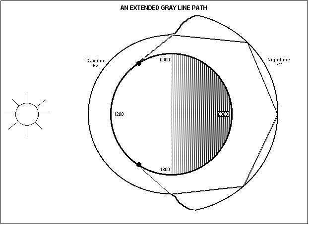
Figure 8. This sketch shows a possible long-path circuit with grazing incidence
hops around the night-time side of the Earth. The signals are launched and retrieved
from the grazing hops by grey line bumps on both ends of the path.
For example, at times contacts are made between Hawaii and South Africa.
The path goes right over Australia and the band is commonly open to
Australia at the same time. To their great frustration, the Australians
hear nothing but excited KH6s. This condition typically occurs around 0800z
(2200 Hawaii, 1800 Australia, and 0900 South Africa).
On the Hawaii end, the signals are launched and retrieved by the equatorial anomaly. The curved surface of the southern edge of the bulge sprays some of the signal down a `low-road' toward Australia, and some of the signal stays up close to the ionosphere and continues on westward on a `high road'.
At the same time, the sunset grey-line bump is over eastern Australia. The high-road signal makes a second chordal hop off the grey line, thus firing the signal into the daylight to the west. By the time the high-road signal comes to Earth the first time, it will have travelled more than 10,000 km - more than 60% of the way to Africa without ever touching the ground. The Australians don't have a chance because the African signals never came to Earth there (most of the time, anyway).
In the case of the Hawaii - South Africa path described above, and the
Hawaii - Spain path described earlier, there may well be another tilted
layer or ionospheric bump that plays a role. Having come 10,000 km on two chordal
hops, if nothing else strange happens, the signal going west still has 6,000 km
to go, requiring at least two conventional daytime hops. However, it will also
pass relatively near the south magnetic pole
in the process.
Satellite measurements of the F-layer near the poles can show significantly tilted layers there, as ions organized themselves along the magnetic field lines that dip nearly to the vertical near the pole. Some of these structures resemble the equatorial bulge, but on a somewhat smaller scale. It is conceivable that these layers might produce a third chordal hop and take the signal all the way to the end of its path before it comes to Earth.
Scatter
Small-Scale Irregularities - Large-scale bumps and ducts are clearly
irregularities in the ionosphere and, as noted, they can cause skip conditions
that are rather different from the simple picture of earth-sky-earth hops. It
is also true that smaller-scale irregularities can produce interesting effects
as well, particularly when they occur in great numbers.
Despite the effort to separate the different effects in this paper and deal with them one at a time, there already have been several references to scatter in the preceding material. This is a consequence of the fact that long-range propagation on six metres often is the result of a combination of effects. Scattering plays a role in many paths; some effects are positive and others negative. In what follows it will become apparent that scattering is inexorably connected to the issue of tilted layers.
In traditional picture of skip, there is a single reflecting or refracting layer of very large horizontal size. Ionospheric scatter differs from skip in that the size of the reflecting or refracting `layer' is usually rather small, but there are many of them. Scattering occurs when a signal encounters a large number of `scattering centres' that are larger than about half a wavelength across.
Each of the individual scatterers can be thought of as a ball-shaped bubble of ionised gas. The sizes of these bubbles might be anywhere from a few tens of meters up to several hundred kilometres. When a radio wave encounters a round bubble, due to the shape the wave is bounced in all directions (not just in one direction as a flat layer would), thus the use of the word `scatter'.
If there is a large number of the scattering centres, then enough of the signal might be reflected to be readable at some distant point. Of course, since these bubbles are all at different distances from the transmitting (and receiving) site, the scattered signals arrive at the receiving site with different phases, leading to a lot of garbling due to massive multipath interference. Moreover, as will be seen, in the ionosphere these centres are normally moving, adding Doppler shift to the witch's brew of funnies.
The ball shape of the scatterers not only reflects the signal in many directions at once, but it also means that, depending on the exact direction of the reflection, there is wide variation in the angle of attack. Everything from straight out and straight back to grazing incidence will be present. Signals going in some directions will have low MUFs and others will have very high MUFs. Thus, while the quality of the signal may suffer due to scattering, it may also make communication possible at VHF.
There are two magnetogeographical regions where ionospheric scatter is fairly common. One is in the magnetic tropics and the other is near the magnetic poles. In the tropics, the effect is intimately associated with the equatorial anomaly and the afternoon fountain. The great ionospheric updrafts that move electrons from the E and F1 regions up into the F2 region produce enormous plumes of turbulent plasma that become aligned with the magnetic field lines. These plumes are composed of a large number of rising bubbles of plasma, in a way looking like a bottle of soda water just after the cap has been removed.
In reality, this is what causes the equatorial bulge. The region within the walls of the bulge is filed with scattering centres. While coherent skip can occur at the lower corners of the bulge, signals entering the bulge itself have significant scattering opportunities. Driven by the afternoon fountain, as one would expect this is basically a night-time effect. Generally speaking, the ionospheric winds in this region cause the plasma to drift eastward. This often adds a systematic doppler shift to the signals.
When this region is probed with an ionosonde (a transmitter that sends signals straight up to measure the critical frequency), instead of the returned signal showing a sharp single F layer echo the display shows a huge diffuse region of echoes ranging from the expected floor of the F layer up to above 800 km. This condition is referred to as spread-F.
Spread-F scattering in the tropics is seasonally enhanced near the equinoxes and negatively impacted by magnetic disturbances. Magnetic storms will completely suppress the effect.
It was mentioned earlier that there are tilted layers near the poles and that some of these look rather like small copies of the equatorial bulge (although their magnetic field alignment in nearly vertical, instead of horizontal like the equatorial region). Here again, one finds spread-F scattering regions.
Near the poles, the scattering centres are often found during the day, as well as the night. The condition is present most of the time, although the equinoxes are favoured. It is less pronounced in the winter and summer months. It seems to be enhanced near solar maximum. This effect is responsible for the heavily modulated signals often encountered in polar crossing paths.
The effect is very rare between 20 and 40 degrees in latitude (north and south). However, it does appear in the mid latitudes poleward of 40 degrees. In this region it is almost always associated with a magnetic storm.
One variation of the scatter picture doesn't involve scattering from ionospheric irregularities at all. Ground backscatter can occur when a traditional ionospheric reflecting layer causes a signal to come back to earth at the end of, say, its first hop. If is strikes a large irregular surface on the ground, for example a mountain range, it may then send some of the signal to skip back in the direction from which it came. This will allow it to be heard by stations that are generally near the transmitting station.
Some Final Comments and Conjectures
The three basic ingredients for a propagation path are ionisation, angle,
and irregularities, in the right combinations. If we restrict our thinking to
the HF spectrum it is easy to explain the bulk of the propagation in terms of
ionisation alone. This is simply because there are generally enough ions to
make some path work at almost any angle. As stated earlier however, at six metres,
F2 usually relies on combinations, and combinations of combinations.
While the bulk of the previous discussion has been focussed on F2, there are a number of ways that a signal can get to, or from, the F layer. For example, if the F-layer ionisation was not quite enough to support the angle for an F2 hop directly from the ground, the partial bending of the wave on the way up by an E-layer cloud (itself not sufficient to cause a reflection) might cause the wave to hit the F layer at a shallower angle and thus produce a high enough M-factor to make the F hop work after all. Similarly, a tilted E-layer could produce the same effect.
On the other hand, a real reflection from an E-layer cloud might skip a signal, originating from a station far from the magnetic equator, and bring it close enough to the equator to take advantage of the equatorial anomaly. Another possibility is the lengthening of a two (or more) hop F2 path by a reflection from the topside of an E cloud in between the two F hops. This avoids the two intermediate passes of D-layer absorption, as well as any scattering of the signal by the ground at the path midpoint.
The role of medium-scale F-layer distortions is very poorly understood. While we often construct pictures of the ionosphere as a smooth spherical surface, this is an idealised picture that cannot account for much of what is commonly seen in six-metre F-layer propagation. The F-layer is a convoluted surface affected by the motion of the subsolar point, ionospheric wind patterns, and even tropospheric weather.
There are a variety of travelling-wave-like structures that are known to exist that can produce moving `ripples' in the ionospheric surface. Similarly, there is evidence to suggest that from time to time there are smaller localised bulges or `domes' not associated with the equatorial anomaly. Any effect such as these that produces tilting in the F layer has the potential to locally raise the MUF because of the `angle of attack' M-factor effect. The sources of these distortions are not clear. When the other contributing factors to the 50 MHz MUF are not quite enough to open the band, these subtle effects, no doubt, can play an important role. But since they relate to a kind of ionospheric weather situation, they are very hard to predict with our present knowledge.
Even random irregularities in the E- or F- layer can have an effect.
These can produce scattering that again can inject (usually weak) signals into the
F layer at angles more suitable for subsequent skipping. Those who
listen
for 48 and 49 MHz television carriers as band condition indicators often
hear signals that arise from the combination of high power and scattering injection.
Summary
When F2 propagation occurs on six metres it is usually the result of the
coincidence of a number of different phenomena that, together, produce suitable
combinations of ionisation levels and radio-wave angles of incidence. Solar
extreme-ultraviolet radiation is the principal source of ionisation. Consequently,
the Sun is the source of many of these effects. However, the full range of operational
factors and their modes of interaction is not known. The diurnal cycle, the
solar activity cycle, solar rotation, solar flares, the equatorial anomaly,
and a variety of terrestrial effects are all known to contribute. Evidence suggests
that there are a number of other poorly understood factors. Various phenomena
that affect the angle of incidence may make more significant contributions to
the basic occurrence of F2 at 50 MHz than at lower frequencies.
So, when is the band open? Well, it is somewhat like playing a slot machine with lots of wheels. There are certain combinations that come up winners to some degree or another. There is an important difference from a slot machine though. The odds of some of the wheels coming up favourable are not entirely random. Within limits, the daily wheel, the solar cycle wheel, and the 27-day wheel are all predictable to some degree. And just to make the game interesting, there are several more wheels we do not know about. In time, we will figure out more of them.
We can say that for stations at magnetic mid latitudes the favoured times are:
Same Hemisphere (North or South)
Daytime, local winter (November to May in the north), near solar maximum,
perhaps during the peak two weeks of the current 27-day cycle, plus unknown
factors.
Transequatorial Paths
Daytime, October-November and March-April, near solar maximum, perhaps during
the peak two weeks of the current 27-day cycle, plus unknown factors.
Not withstanding these patterns, it is obvious that this is truly an unfinished story. Even though the list above addresses the most probable times, it is clear that F2 can pop up at any time, even as a result of a flare at solar minimum. Many openings have happened when none of these conditions were known to be present. This only goes to underscore the importance of the unknowns and to present a challenge to the community to keep listening. One thing that is known for certain: you can’t work them if your radio is off.
Some References
Ionospheric Radio, Kenneth Davies, Peter Peregrinus Ltd., London,
1990
Introduction to Ionospheric Physics, Henry Risbeth and Owen K. Garriott,
Academic Press, New York, 1969
Ionospheric Radio Waves, Kenneth Davies, Blaisdell Publishing Company,
Waltham MA, 1969
Notes:
* The Gemini Observatory is operated by the Association of Universities
for Research in Astronomy under a cooperative agreement with the National Science
Foundation.
** “Angle of attack” is a borrowed aeronautical term. It is the angle between the ionosphere and the direction of travel of the radio wave. Although I prefer this particular way of looking at it, usually physics texts use its near relative, the “angle of incidence”. This is the angle between the vertical with respect to the ionosphere and the direction of the wave, that is to say (90° - angle of attack). The equations change a little, but the answers are the same.