by Gary Hyde, G7LXK1. Introduction
This paper is a reply to "A Hidden Mode of Sporadic-E ?" by Volker Grassmann [1]. It is shown that the interpretation of a minor peak as ‘double scatter’ is unlikely, and the double-peaked distribution is what one would expect, taking into account the known properties of Es and the geography. There is no need to invoke a ‘Hidden Mode’.
2. The Problem
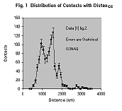 The
anomaly reported in [1] is a double-peak in the distance distribution of 50 MHz
Es contacts, worked from several sites in NW Germany. Figure 1 reproduces as
closely as possible ([1], figure 2). The two peaks are referred to as Es(SS) and
Es(LS), respectively Short Skip and Long Skip. However, the behaviour of these
two peaks shows no significant difference with time of day, direction or months
of activity ([1], section 3.1). It is difficult to comment on the differences
observed [1] in the ratio of SS and LS during the season without seeing these
distributions. However, it would be expected that the maximum electron densities
would be higher mid-season, so the proportion of Es(SS) would also be greater at
this time; this seems to be consistent with the observations reported in [1].
The
anomaly reported in [1] is a double-peak in the distance distribution of 50 MHz
Es contacts, worked from several sites in NW Germany. Figure 1 reproduces as
closely as possible ([1], figure 2). The two peaks are referred to as Es(SS) and
Es(LS), respectively Short Skip and Long Skip. However, the behaviour of these
two peaks shows no significant difference with time of day, direction or months
of activity ([1], section 3.1). It is difficult to comment on the differences
observed [1] in the ratio of SS and LS during the season without seeing these
distributions. However, it would be expected that the maximum electron densities
would be higher mid-season, so the proportion of Es(SS) would also be greater at
this time; this seems to be consistent with the observations reported in [1].
Consider the distribution given in figure 1. A range of Es height from 90 to 120 km implies a maximum single hop range of between 2130 and 2450 km ([2], p.2-43). This is indeed where the plot goes to zero. The number of contacts beyond this distance is small enough to be statistically compatible with a normal double hop distribution. Therefore to call this a ‘hidden mode’ already seems to be a little too sensational. The problem may be posed in a less dramatic way; that is, why does the otherwise normal distribution of Es contacts on 50 MHz from this area apparently show two preferred ranges?
3. Double Hop in the Two Mode Hypothesis
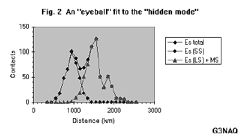 First
consider the supporting claim [1] that the minor peak at 1800 - 1900 km
represents double hop "SS". In figure 2 the two modes are separated
into two distributions, the "SS mode" and the remainder, which
represents predominantly the "LS mode" plus multi-skip (MS). This was
done empirically (an ‘eyeball fit’ rather than by computer), but the
resulting distributions look convincing.
First
consider the supporting claim [1] that the minor peak at 1800 - 1900 km
represents double hop "SS". In figure 2 the two modes are separated
into two distributions, the "SS mode" and the remainder, which
represents predominantly the "LS mode" plus multi-skip (MS). This was
done empirically (an ‘eyeball fit’ rather than by computer), but the
resulting distributions look convincing.
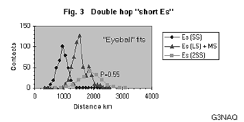
Using figure 2, the double hop distribution of the "SS mode" may be estimated by doubling the distance scale and applying a double hop ‘probability coefficient’ P to the number of events in each bin. Figure 3 shows the results with P = 0.55 to make the height comparable to the peak. This value of P is very high, but it is evident that whatever value of P is used, the calculated distribution can not satisfactorily reproduce the observed distribution. The minor peak is much too narrow to represent the distribution of double hop SS events as claimed [1].
<pic 11 about here>
4. Distribution of Land Area
If the claims of [1] are true, we must show that the distribution is not due to variations of land area with distance. Looking at the map of Europe, intuitively it looks as the proportion of sea to land increases significantly at around 1200 km. In defence ([1], figure 6: ‘Sea, land and coastal terrain areas as a function of distance in reference to JO40DF’) was produced.
This figure is difficult to interpret because (i) the division is into sea, land, and ‘coastal areas’, without defining the latter - surely the only relevant division is between habitable land and sea; (ii) the shape of the plot is dominated by the term proportional to R, making it difficult to assess; (iii) the way it is drawn with a long distance axis and short event axis tends to minimise any deficiency; (iv) it has obvious errors, since in some bins (e.g. 600 - 700 km) the total does not add up to what it should be (the ‘True’ line). It was therefore decided to check this work, approaching it in a different way.
 Since
the number of contacts made from the three different locations which contribute
to the data in [1] were not known to the author, the geometric centre of the
three locations was estimated; it turns out to be near the city of Kassel. This
position was used as the centre for the following evaluation. However, the
conclusion is not expected to be sensitive to the exact choice of position.
Since
the number of contacts made from the three different locations which contribute
to the data in [1] were not known to the author, the geometric centre of the
three locations was estimated; it turns out to be near the city of Kassel. This
position was used as the centre for the following evaluation. However, the
conclusion is not expected to be sensitive to the exact choice of position.
It is a difficult and time consuming task to accurately divide up the map of Europe into small squares, and then count them, as DF5AI has described. I therefore drew radial lines at 20 deg intervals and circles in 100 km steps, then measured with a protractor the angles between points where land changed to sea and the reverse. This gave the fraction of the total 360 degrees which was land as a function of distance. The theory of Calculus tells us that the area A can then be estimated, since dA = 2 p R df dR, where R is the distance and F is the azimuth angle.
Figure 4 shows the distribution of land as a percentage of the azimuth in range R steps of 100 km. Also shown is this plot multiplied by the circumference C = 2pR, which is then proportional to the area; this has been scaled by an arbitrary constant k to bring it on the same scale. For comparison, the distribution of contacts is also shown, scaled by a factor 0.5 for the same reason. The proportion of land to sea does indeed drop around 1350 km, but not sufficient to explain the drop in contacts.
5. The Distribution of Es
 Another
factor determining contacts made is the geographic distribution of Es. Largely
due to the extensive deployment of ionosondes during the International
Geophysical Year (1958), the world-wide distribution of Es has been determined.
The source used was a map giving contour lines of the percentage of time the Es
critical frequency foEs (the highest frequency which is reflected back to earth
from the ionosphere at vertical incidence) exceeds 7 MHz during the Es season,
that is May, June, July, and August [3]. The frequency of 7 MHz may at first
seem irrelevant to 50 MHz propagation, but the maximum frequency reflected to
ground (MUF) increases rapidly with decreasing angle of incidence. A radio wave
emitted at zero degrees elevation angle will meet the E layer at 100km at an
angle of 79.2 degrees to the normal. The secant law would predict the MUF to be
7 sec(79.2) = 37 MHz. However, the secant law is known to under-estimate the MUF
for Es by a factor of between 1.25 and 1.5 [2,3]. Thus this corresponds
approximately to 50 MHz propagation.
Another
factor determining contacts made is the geographic distribution of Es. Largely
due to the extensive deployment of ionosondes during the International
Geophysical Year (1958), the world-wide distribution of Es has been determined.
The source used was a map giving contour lines of the percentage of time the Es
critical frequency foEs (the highest frequency which is reflected back to earth
from the ionosphere at vertical incidence) exceeds 7 MHz during the Es season,
that is May, June, July, and August [3]. The frequency of 7 MHz may at first
seem irrelevant to 50 MHz propagation, but the maximum frequency reflected to
ground (MUF) increases rapidly with decreasing angle of incidence. A radio wave
emitted at zero degrees elevation angle will meet the E layer at 100km at an
angle of 79.2 degrees to the normal. The secant law would predict the MUF to be
7 sec(79.2) = 37 MHz. However, the secant law is known to under-estimate the MUF
for Es by a factor of between 1.25 and 1.5 [2,3]. Thus this corresponds
approximately to 50 MHz propagation.
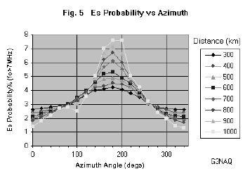
 To
estimate the effect from NW Germany, the contours were redrawn on a map of
Europe and the value assessed by linear interpolation, again at intervals of 20
degrees in azimuth and 100 km in distance, between 300 and 1000 km. Figure 5
shows this data plotted against azimuth angle for each radial distance. As can
be seen, the distributions peak as expected close to the southerly direction
(180 degrees), and show an increasing tendency to do so with increasing
distance. The distributions are not entirely symmetric, however, because of the
skewed contours and the presence of an anomaly roughly centred near the western
shore of the Black Sea. This ‘hole’ in the occurrence of Es would produce a
dip in the number of contacts beyond 2000 km in this direction, but is too far
to explain the closer distribution.
To
estimate the effect from NW Germany, the contours were redrawn on a map of
Europe and the value assessed by linear interpolation, again at intervals of 20
degrees in azimuth and 100 km in distance, between 300 and 1000 km. Figure 5
shows this data plotted against azimuth angle for each radial distance. As can
be seen, the distributions peak as expected close to the southerly direction
(180 degrees), and show an increasing tendency to do so with increasing
distance. The distributions are not entirely symmetric, however, because of the
skewed contours and the presence of an anomaly roughly centred near the western
shore of the Black Sea. This ‘hole’ in the occurrence of Es would produce a
dip in the number of contacts beyond 2000 km in this direction, but is too far
to explain the closer distribution.
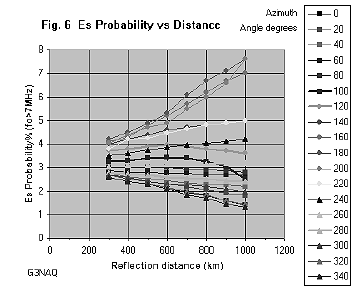
Alternatively, one can plot these values as a function of distance, for each azimuth angle. This is shown in figure 6; the effect of the anomaly can be easily be seen at 100 degrees angle.
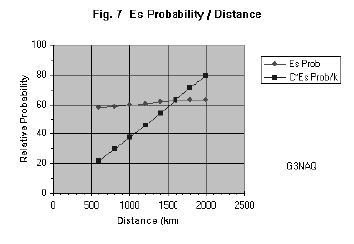 To
assess the total effect on the distance distribution, the values at each radius
were added for all angles, and plotted against distance. This time the distance
axis was doubled to represent the range of the contacts; with a strong
propagation mode like Es it is safe to assume specular reflection, and indeed
this has been shown to be the case [2,3]. This distribution is shown in figure
7. This shows a trend of slowly increasing probability with distance up to about
1900 km. Again the scaled curve is also shown after multiplying by C=2pR.
To
assess the total effect on the distance distribution, the values at each radius
were added for all angles, and plotted against distance. This time the distance
axis was doubled to represent the range of the contacts; with a strong
propagation mode like Es it is safe to assume specular reflection, and indeed
this has been shown to be the case [2,3]. This distribution is shown in figure
7. This shows a trend of slowly increasing probability with distance up to about
1900 km. Again the scaled curve is also shown after multiplying by C=2pR.
6. Combining the Distributions of Land Area and Es Probability
So far the distribution of Es probability and land area have been considered separately, and have failed to explain the observed double-peaked distribution of single hop Es. However, properly these two distributions should be combined. It is clear from the azimuth plot of Es probability (figure 6) that the land/sea distribution to the south is much more important than that to the north, and to a lesser extent, to the east and west.
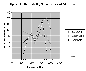 To
put this into effect, I formed a matrix corresponding to each point of my
azimuth/distance table containing Es probability. Since the relevant land is at
double the distance of the Es reflection point, I looked at this distance along
the same azimuth line, and entered in the matrix a 0 if this point corresponded
to sea, or 1 if it corresponded to land. I then multiplied each cell of the two
matrices, thus all the probabilities corresponding to points which fell in the
sea were set at zero, the others remaining at their previous values. Then I
repeated the exercise of summing the probabilities at all azimuth angles for
each distance; these results are shown in figure 8. The appearance of a drop of
suitable magnitude at the required distance is quite evident.
To
put this into effect, I formed a matrix corresponding to each point of my
azimuth/distance table containing Es probability. Since the relevant land is at
double the distance of the Es reflection point, I looked at this distance along
the same azimuth line, and entered in the matrix a 0 if this point corresponded
to sea, or 1 if it corresponded to land. I then multiplied each cell of the two
matrices, thus all the probabilities corresponding to points which fell in the
sea were set at zero, the others remaining at their previous values. Then I
repeated the exercise of summing the probabilities at all azimuth angles for
each distance; these results are shown in figure 8. The appearance of a drop of
suitable magnitude at the required distance is quite evident.
7. Conclusion
It seems that a combination of the known geographic distribution of Es, combined with the land/sea distribution, is sufficient to explain the observed anomaly in the distance plot. Of course, all the factors influencing this curve have not been taken into account; in particular, this curve should be similarly convoluted with the distribution of amateur activity on 50 MHz. Apart from the difficulty of obtaining this data, it appears not to be necessary for present purposes. The aim was not to reproduce exactly the distribution given in figure 1, but to show that no new propagation properties are involved.
References
[1] V. Grassmann DF5AI, "Hidden Mode of Sporadic-E? More Magic with the Magic Band", submitted to UKSMG 16 Oct 1999.
[2] I.F. White G3SEK (ed.) "The VHF/UHF DX Book" (DIR Publishing 1992): G. H. Grayer G3NAQ, Chapter 2, "VHF/UHF Propagation". ISBN 0 9520468 0 6.
[3] E. K. Smith Jr., S. Matsushita (eds.) "Ionospheric Sporadic E" (Pergamon 1962): H.I. Leighton, A.H. Shapley, E.K. Smith Jr. "The Occurrence of Sporadic E during the IGY" pp.166-177;